Connections between data augmentation and out-of-distribution data through the lens of KL divergence

August 2025•16 min read•~2,600 words

Diego Huerfano

CEO & Co-founder
Nabla Labs

Data augmentation is a non-negotiable common practice when training ML and deep learning models. After all, the goal seems to be simple and only full of benefits: simulate plausible new data points from the available ones in the training set so that the model generalizes better, is more robust to noise in the data, has a larger context of what similar samples look like and so on. Another effect of this process is the reduction of out-of-distribution data (OOD) that the models are exposed to at inference time.

The intuition tells us that the more aggressive the data augmentation is, the less likely a given data point will be considered as OOD at inference time. In this post, we'll see how this intuition can be understood from a formal, mathematical perspective. While I don't claim that this framework fully and accurately describes the relation between data augmentation and OOD, after making the usual assumptions we arrive to it in a natural way. For examples where theory meets practice in a similar way, I like remembering the case in stable diffusion literature where a formalization of scored-based generative models as SDEs allowed for a derivation of the more simpler ODE [1], now a practical standard in the field.

How Are the Data and Empirical Distributions Mathematically Defined?

The framework for machine learning is to assume the data is drawn from a hypothetical distribution that is mainly defined by the application domain and how the data is collected, the data generating process. This process is specified by a random variable Loading...that follows the data distribution, Loading..., and the data collection process consists of drawing a sequence Loading... of length Loading...so that the variables are independent and identically distributed (IID), i.e. Loading.... The result of data collection is a sample Loading..., e.g. in the case of images, each image Loading... is a realization of the random variable Loading.... Although the data distribution Loading... is unknown and complex, it's assumed that it exists and that it drives the data in the described way. It's the way how we link the reality to the theory.

The empirical data distribution [2] is the observed distribution of a sample drawn form the data distribution. Let the sampleLoading... (that can be e.g our training or test set), its empirical distribution is defined by the density

where Loading... is the Dirac delta function. As simple as just being an average of individual single-point densities, the Dirac delta functions centered at each data point Loading..., it is a good approximation of the true data density Loading...when the sample size Loading... is large enough.

How Does Data Augmentation Affect the Empirical Data Distribution?

If our traning dataset is Loading..., during traning we apply a data augmentation transformation Loading... (parametrized by Loading...), to each data point Loading... that results in a new random variableLoading.... The nature of this transformation depends on the domain and the task we are trying to solve but often involves perturbing each Loading...in a way that Loading... is equivalent to Loading...for the task, e.g. the image class of both augmented and original data points is the same in an image classification task. This is important because it restricts how far the augmented points can end up from the original points, so that Loading...is not too large to the extent that Loading... lies closer to another data point of a different class or that the features of Loading... are just meaningless (too noisy) for the task, for example.

Visualization of data augmentation: original data points and their Gaussian-augmented distributions in feature space — **Figure:** Visualization of data augmentation in machine learning. Black dots represent original data points Loading..., while blue points and contours show the effect of the augmentation densities Loading... in feature space.

The augmentation Loading...induces then a probability density Loading... of augmented samples around each Loading...that is in principle known to us as we have control over Loading.... Ideally, Loading... is high around Loading...and low when we are far from Loading... (see Figure). For example, if the augmentation consists of adding randon gaussian noise to the image Loading...,Loading... is a gaussian distribution centered at Loading...with a standard deviation defined by Loading.... In the end, we obtain the augmented empirical density

that, similarly to the empirical density, is an average of densities around each data point where the Dirac delta functions have been spread out to Loading... by means of the augmentation.

Quantifying the Data Drift

After training, we have an inference dataset Loading...with empirical density Loading.... The standard way of quatifying the dataset drift is to use the Kullback–Leibler divergence [3] between the inference data distribution Loading... and our augmented data distribution Loading..., given by

(using the fact that the delta function simplifies the integral to a evaluation of the integrand). As always, an equation is more than just symbols and this one confirms the following insights:

For out-of-distribution points Loading..., i.e. points that are far from all the training data points, Loading... is close to zero and so will push the divergence to infinity, as expected. This means that we are using the trained model on a dataset that is not representative of the training data distribution and the augmentation transformation, resulting in poor performance.
The opposite of the above is also true: large divergence only occurs when there is at least oneLoading... far enough from the training data.
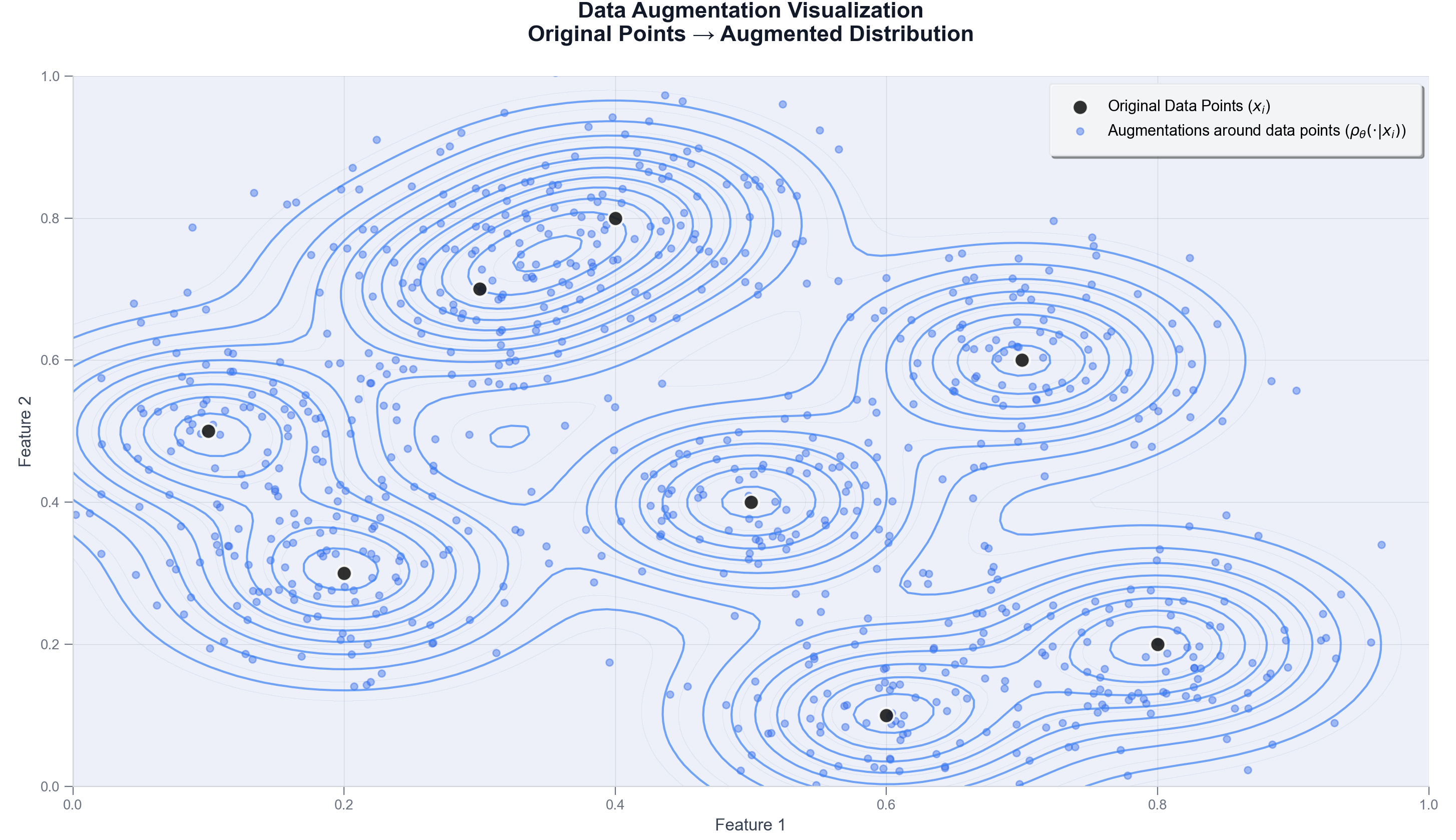
The augmentation Loading... controls the spread of Loading...around each training data point Loading... and in turn defines what is considered out-of-distribution: If the augmentation is aggressive, the spread of Loading...will be large and so the the only out-of-distribution points will be the ones that are very far from the training data. If the augmentation is conservative, Loading...will be over-concentrated around each Loading....
This analysis supports out-of-distribution detection methods [4] based on the direct relationship between the distance to in-distribution points and the probability of being out-of-distribution.

Key Takeaways

From spikes to mixtures: Augmentation replaces Dirac deltas at each training sample with local densities around them, so models learn from neighborhoods rather than isolated points.
OOD = low augmented mass: A test point is out-of-distribution when the total augmented mass it sees from the training set is small (the sum of densities around it is near zero).
KL makes this explicit: The divergence depends on log of the summed augmented densities at each test point and is driven by samples with little nearby training mass.
θ is a deployment knob: Stronger augmentation widens what counts as in-distribution; too weak yields brittle models, too strong can blur classes and add noise.
A principled view of “tricks”: Thinking in terms of augmentation densities lets you compare different transforms by how they spread probability mass around data.

Frequently Asked Questions

What changes from the empirical distribution to the augmented one?

The empirical distribution is a sum of Dirac deltas at observed samples. Augmentation turns each delta into a local density around the sample and the whole dataset into a mixture of those densities, so models learn from neighborhoods rather than isolated points.

How does this explain out-of-distribution (OOD) behavior?

A test point is OOD when the total augmented probability mass it receives from the training set is small — i.e., the summed densities around it are near zero. Those points dominate the divergence and often correspond to poor model performance.

Where does KL divergence fit in this picture?

In this setup the KL term depends on the log of the summed augmented densities at each test point. Large KL values arise from test samples with little nearby training mass, giving a quantitative way to audit dataset shift.

How should I choose the augmentation strength θ?

Treat θ as a deployment knob: stronger augmentation widens what counts as in-distribution; too weak yields brittle models; too strong can blur class boundaries and add label noise. Tune θ with validation data that reflects realistic deployment perturbations.

References

About Diego Huerfano

He has an academic background in pure mathematics and professional experience in perception systems for autonomous vehicles as well as in industry applications of human-body understanding. He is currently commited to exploring connections between theoretical, generative frameworks and their practical applications in the field of computer vision.

Synthetic Data GenerationDeep LearningStatistical ModelingGenerative AIGenerative ModelingComputer Vision

Connect on LinkedIn

Contact Author

References

- Song, Y., Sohl-Dickstein, J., Kingma, D. P., Kumar, A., Ermon, S., & Poole, B. (2021). Score-Based Generative Modeling through Stochastic Differential Equations. arXiv:2011.13456 [cs.LG].
- Empirical distribution function (Wikipedia)
- Kullback–Leibler divergence (Wikipedia)
- Sun et al., “Out-of-Distribution Detection with Deep Nearest Neighbors” (ICML 2022)